Coaxial cable stubs (2nd part)

From my original post of 12-04-2010, on Hamradioweb.org.

Last week, readers who have glanced at my previous post will probably have gone around the web in search of more information.

 A stub:

 Let’s quickly see what lengths are generally used to construct stubs; these measurements refer to cables with a speed factor of 0.66, such as RG58 or 213.

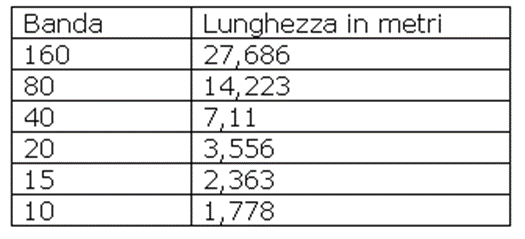
 In the table above we find the finite lengths of the ¼ wavelengths of each HF band (excluding WARC) taken at the beginning of the band. Of course, due to the imperfection of the materials in use, these measurements are only approximate and subject to customisation according to the frequency we would like to be more attenuated.
 Therefore, in order to avoid unpleasant inconveniences and ending up with a cable that is too short, the advice is to cut the cable slightly longer than the recommended/calculated measurement, in percentage terms it is advisable to abound from 5%, on 160 metres, up to 10%, on the 10-metre band.

 A further table, which may be useful when cutting and calibrating coaxials, may be as follows:

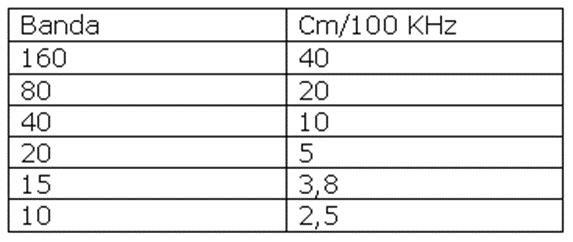
 Based on the band, it is possible to determine how much to cut to reach the desired frequency; for example: on the 80 each 20 cm of cut cable will affect the frequency response rise by 100 KHz.

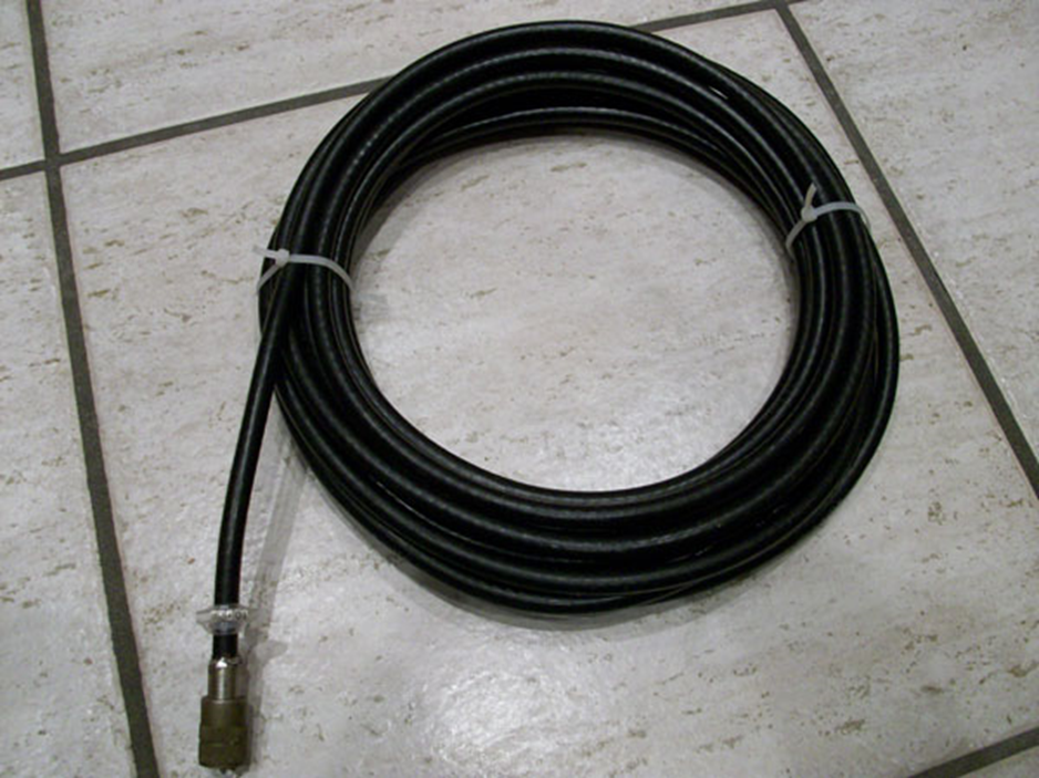
 Preparing a coaxial stub is very simple: just lay the cable as straight as possible and measure it with a metric tape, preferably longer than the cable stub itself.
This will prevent you from measuring errors: measuring a stub for 160 with a 2 metre tape measure is not convenient and can introduce errors, especially if you are alone doing the work.

 The final frequency will also be affected by the stub used to connect to the T on the transmission line, but the calibration will still be done with the PL soldered to the cable.

 The other end of the cable, the open or shorted end, must always be treated with care. In the case of an open stub, when making the calibration cut, it is convenient to strip the braid about 1 cm shorter than the central insulator and the central conductor itself. In the case of a DC stub, during calibration, it is possible to temporarily short the centre conductor and the braid, even by winding them together; when the desired frequency is reached, the braid and the centre conductor must be well soldered for better system performance. Once the work is completed, the terminal should be protected, possibly with a heat-shrink
sleeve or a few turns of good insulating tape.

Calibration

 The best way to calibrate a stub is to use a VNA (Vector Network Analyzer). Unfortunately, not everyone has such a device, so if you don’t have one or don’t have friends who can lend it to you, we will see how you can fall back on other systems, unfortunately a little less reliable.

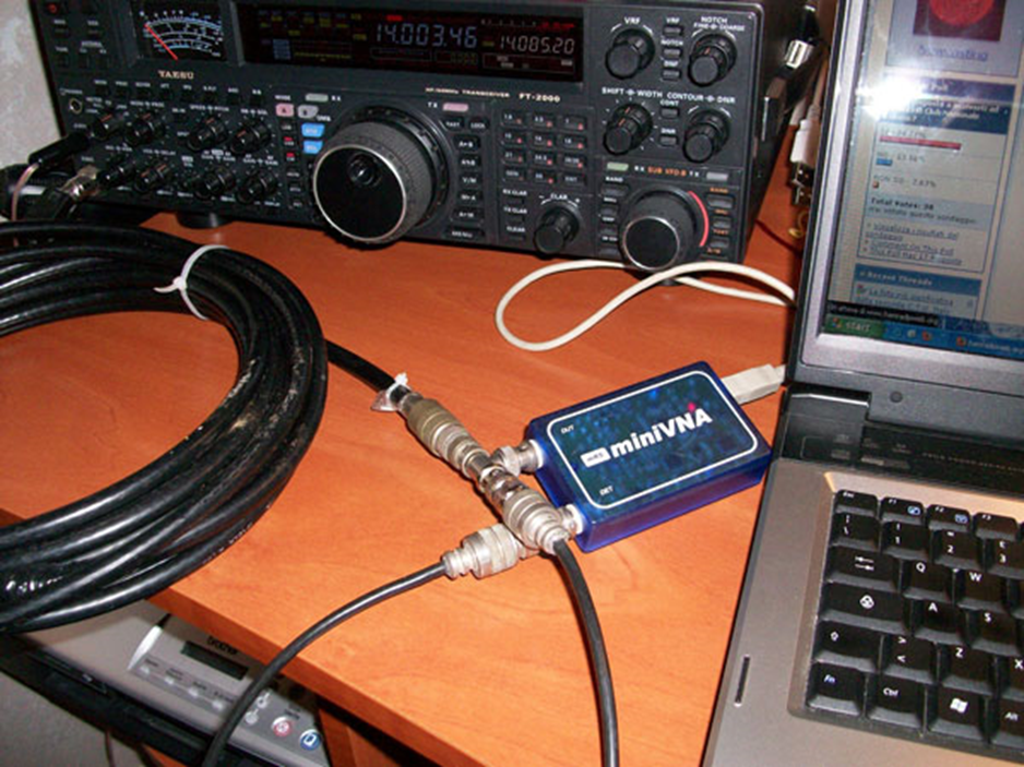
 I personally use the miniVNA, even the graphs you see in the posts are taken in real time from one of its management software.

 From the photo above we can see the application of the miniVNA for the calibration of a stub for 20 and 10 metres (attenuates 40 and 15 metres), then a ½ wave open for the 20.
To the DUT port is applied the central connector of a T, on one side of the T is connected the stub while on the other a piece of coaxial in turn connected to the DET port. We put the miniVNA software into transmission mode by displaying the HF band 1-30 MHz, activate single or continuous swap from the software, and we will see the following graph appear on the screen:

 Of course, this graph refers to an already calibrated stub.
I would like to add a note in this regard: in this case the two attenuation maxima do not fall exactly in the two desired bands, i.e. 40 and 15 metres, this is because if we centre the 40 band we will have the attenuation of the 15 on the upper part of the band itself, in the same way if we centre the attenuation of the 15 metres we will find the first notch below 7 MHz. So with a single stub we have to juggle the best point where to make it work.

 A second method, which in practice is similar to the one seen now, can be carried out if we have a tracking generator and a spectrum analyser.

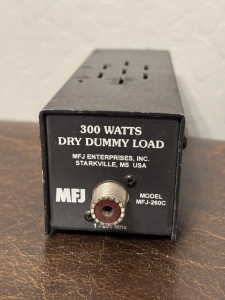
 The simplest method of measurement, although less precise, can be carried out with a transceiver or antenna analyser and a dummy load.
From what we have read so far, we have seen that on the frequency of use, the stub has a very low SWR, which can help us find the right working frequency.
We want, for example, to calibrate a stub for 20 metres like the previous one. At the antenna connection of an antenna analyser or transceiver, we place the central connector of the usual T, on one side we place the stub and on the other a 50 Ohm dummy load (even a 47 Ohm resistor is fine).
With little power (in the case of a transmitter) we start to find the point where we find a flat SWR: practically at 1 (if the RTX does not have an internal ROSmeter of course use an external one). Usually this flat curve, at the start of operations, is lower than the 20m frequency because the coax is longer. By cutting the stub a few centimetres at a time, we are able to bring it into resonance on the 20-metre band with a fairly high degree of certainty of bringing the maximum attenuation to the desired frequency.
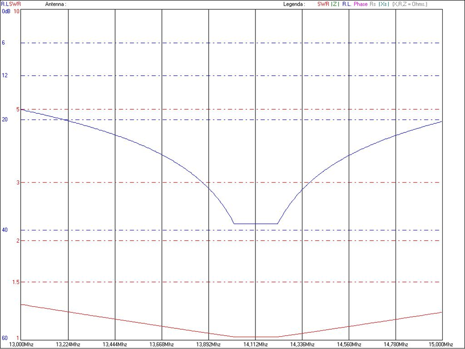
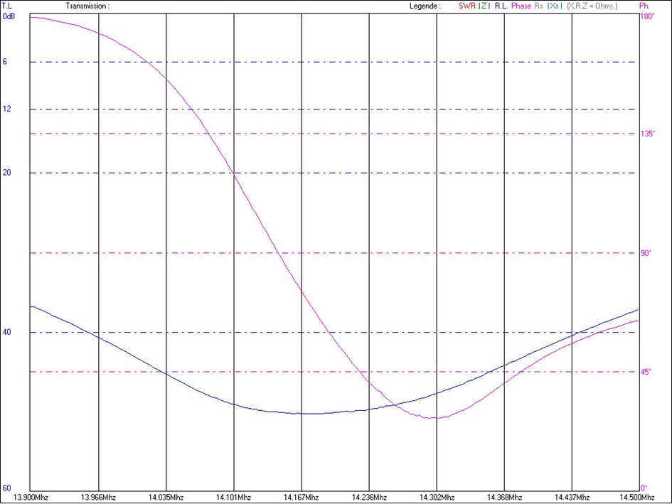
The graph below shows the SWR (red line) of the 20 stub at 14 MHz. This is flat for a good portion of the band. The blue line is the return loss.

 If we have a second rtx or receiver, we can check with the S-meter the depth of the stub attenuation by transmitting on the 40 band spectrum and receiving on the 20 the second harmonic beat attenuated by the stub.

 Below we have a table from which we can observe the most commonly used stubs:

Stub couplings

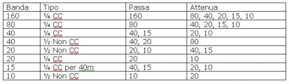
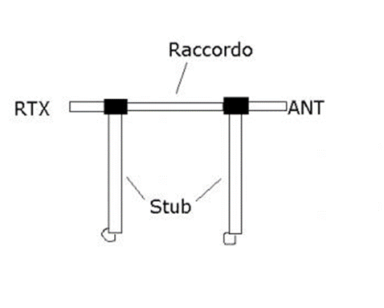
 To increase the attenuation of unwanted signals, two stubs can be placed in parallel along the transmission line.

 Let us now see how two ¼-wave DC stubs behave.

 The coupling of two stubs must be carried out with some knowledge, in fact, placing two stubs, one immediately after the other, does not give the desired effect, yes it increases attenuation, but it does not guarantee maximum efficiency. Another belief is that placing a ¼-wave section of cable on the fundamental frequency between two stubs of this type guarantees maximum performance.
 The discourse, unfortunately, is not easy to deal with, because if, on the one hand, an appropriate length of coupling cable optimises the attenuation on the 2F (second harmonic), on the other hand we may notice little improvement on the 4F and so on.

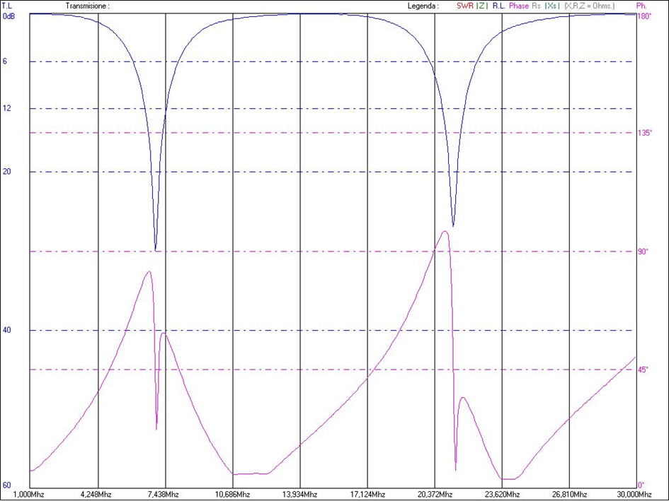
 Another issue that must be addressed, in order to obtain the desired results, concerns the calibration of the individual stubs. The maximum attenuation will be obtained if the two stubs are cut for exactly the same frequency; usually, if the attenuations fall on the same frequencies, depending on the length of the connection joining the stubs, we can see a doubling of the attenuation plus about 6 dB of additional attenuation. The following is a graph of two ¼-wave stubs for the 40 meter, showing the attenuation on the 2F, i.e. the 20 metres.

The connection of the two stubs was made with a piece of 1/6-wave cable. The attenuation at 14.170 is about 50 dB and not about 60 as one would expect, this is because the two stubs were not cut for the same frequency but for slightly different frequencies. In this way, it is possible, at the expense of a less pronounced negative peak, to cover the entire band with an attenuation that is still considerable.
Care must be taken not to exaggerate by having the two stubs resonate at too different frequencies, as this could result in a doubling of negative peaks along the band to be protected and a deterioration of overall performance.
The choice of how to cut the two stubs depends on the use to be made of them.

 The following table shows the relative attenuations when coupling two stubs of the type now discussed according to the length of the coupling cable:

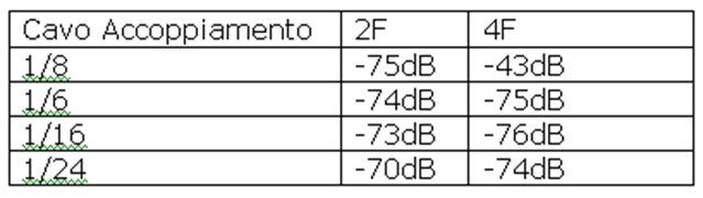
 Of course, the values are only guidelines, they give a sense of how much the attenuations vary according to the length of the cable used to connect the two stubs
 As far as open ½-wave stubs are concerned,
on the other hand, things are considerably simplified. As we saw last time, in the table of single stub efficiencies, open stubs perform better with the same cable type and length than DC stubs. Again, coupling two ½ wave stubs gives better performance. By using a ¼-wave long coupling cable on the sub-harmonic, we generally obtain double the attenuation plus about 6 dB more. For example, if we create a double stub to pass the 20 and attenuate the 40, the length of the coupling cable must be ¼ wave to the 40 metres and not the 20.
Even in this case, it is possible to calibrate the two stubs to slightly different frequencies to cover the entire band.

 In both cases, the first stub is calibrated individually, then the entire system is connected and the second stub is calibrated.

 There would be more to say about stubs, but my task ends here for now. I remain available for questions and suggestions.

 Thank you for your attention.